Basic RAG

Introduction

• Large Language Models (LLMs) are good at writing fluent answers, but they only “know” what was in their training data. They can also hallucinate — invent facts that sound confident but are wrong.
• RAG (Retrieval-Augmented Generation) is a simple idea: before the model answers, we retrieve relevant documents from a knowledge base, then ask the model to generate an answer using those documents as context.
• Think of it like an open-book exam. Without RAG, the LLM answers from memory. With RAG, it can look up the right pages first, then write the answer.

Why RAG matters

• Up-to-date information: You can add new PDFs, notes, or web pages without retraining the whole LLM.
• Private / domain data: Course notes, company docs, or research papers that were never in the model’s training set.
• More grounded answers: The model is steered by retrieved text, so answers can cite or stick closer to your sources.

The basic RAG pipeline

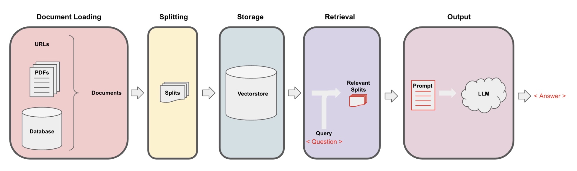
A minimal RAG system usually has four steps:

1. Ingest — collect documents (PDF, Markdown, text, etc.).
2. Chunk — split long documents into smaller pieces so search stays precise.
3. Retrieve — convert the user question into a vector (embedding), then find the most similar chunks in a vector store.
4. Generate — send the question + retrieved chunks to an LLM and get the final answer.

User question
    |
    v
[Embedding + search] --> top-k relevant chunks
    |
    v
[LLM prompt: question + chunks] --> answer

• In short: Retrieve first, then generate. That is the core of basic RAG.

Step by Step Coding guide:

• The following code using langchain version 1.2.8. The code might be changed if you switch between different langchain version.

Step 1: Ingest/Load Documents

• Here we use PyPDFLoader and DirectoryLoader to load single/multiple pdf files

from langchain_community.document_loaders import PyPDFLoader, DirectoryLoader   
loader = DirectoryLoader(
    "mdocs",
    glob="*.pdf",          # match PDFs (use ** for recursion)
    loader_cls=PyPDFLoader,   # use PyPDF for each matched file
    show_progress=True,
    use_multithreading=True,
    max_concurrency=8,
)

docs = loader.load()
print(len(docs), docs[0].metadata)

• Other supported format are: TextLoader for txt file or other text based like python file, or Docx2txtLoader for MS Word files

Step 2: Split loaded documents into chunks

• LLMs and embedding models can only process a limited number of tokens (a token ~ 3/4 of a word) at a time.
• Long PDFs often exceed that limit, so we split the text into smaller chunks before indexing and retrieval.
• We will use RecursiveCharacterTextSplitter for this task. (In addition, you can also use other splitter method like TokenTextSplitter, CharacterTextSplitter)

from langchain_text_splitters import RecursiveCharacterTextSplitter

• Before splitting, we set two important parameters:
  • chunk_size: the maximum length of each chunk (here measured in characters). Smaller chunks make search more precise; larger chunks keep more surrounding context.
  • chunk_overlap: how many characters are shared between neighboring chunks. Overlap reduces the chance that a sentence or idea is cut in half at a chunk boundary.
• Rule of thumb: start with a modest overlap (often about 10–20% of chunk_size). For a quick demo we use small values; for real PDFs you often use larger sizes (for example chunk_size=1000, chunk_overlap=200).

chunk_size = 26
chunk_overlap = 4

r_splitter = RecursiveCharacterTextSplitter(
    chunk_size=chunk_size,
    chunk_overlap=chunk_overlap
)

splits = r_splitter.split_documents(docs)
print(len(splits), splits[0].page_content[:200])

Step 3a: Embed chunks and retrieve similar text

• Retrieve means: turn text into numbers (embeddings), store those vectors, then for a new question find the chunks whose vectors are closest (most similar in meaning).
• An embedding is a list of numbers that represents the meaning of a piece of text. Similar sentences land near each other in that vector space.
• A vector store is a database for those embeddings. For a basic local demo we use FAISS (you can also use Chroma, LanceDB, etc.).

from langchain_community.vectorstores import FAISS
from langchain_ollama.embeddings import OllamaEmbeddings
oembedding = OllamaEmbeddings(model="mxbai-embed-large:335m")  

db_faiss = FAISS.from_documents(
    documents=splits,
    embedding=oembedding
)
db_faiss.save_local("docs/faiss_new")

• Ask a question and pull the top-k most similar chunks:

query = "What is the main topic of the document?"
docs_and_scores = db_faiss.similarity_search_with_score(query, k=5)

for i, d in enumerate(docs_and_scores):
    print(f"--- chunk {i+1} ---")
    print(d.page_content)
    print(d.metadata)

• What just happened:
  1. The query was converted to an embedding with the same model used for the chunks.
  2. FAISS compared that vector to all stored chunk vectors.
  3. It returned the k=5 closest chunks — these become the context for the LLM in Step 4.
• Tip: if results look weak, try a larger chunk_size, a different embedding model, or a clearer query. Retrieval quality drives RAG quality.

Step 3b: Reranker

• Vector search is fast, but the top-k list is not always perfectly ordered. A chunk can be “nearby” in embedding space and still be a weak match for the exact question.
• A reranker is a second, more careful model. It looks at the question and each candidate chunk together, scores how well they match, then reorders (or drops) chunks before we send them to the LLM.
• Simple picture:

Question
   |
   v
FAISS retrieve many candidates (e.g. top 20)   <-- fast, approximate
   |
   v
Reranker scores each (question, chunk) pair     <-- slower, more accurate
   |
   v
Keep the best few chunks (e.g. top 5) --> LLM

• Why use it: better context for generation, fewer irrelevant chunks, often fewer hallucinations from noisy retrieval.
• Trade-off: reranking adds compute time, so we usually retrieve a larger k first, then keep a smaller final set.

from sentence_transformers import CrossEncoder
reranker = CrossEncoder("cross-encoder/ms-marco-MiniLM-L-6-v2")

pairs = [(query, d[0].page_content) for d in docs_and_scores]
scores = reranker.predict(pairs)

reranked_docs = [
    doc for _, doc in sorted(
        zip(scores, docs_and_scores),
        key=lambda x: x[0],
        reverse=True
    )
]

top_docs = reranked_docs

Step 4: Generate

• Generate is the last step: we give the LLM the user question plus the retrieved (and reranked) chunks as context, and ask it to answer using that context.
• Without this step, RAG is only search. With it, the model writes a fluent answer grounded in your documents (the open-book part of the exam).
• Keep the prompt simple for beginners: instruct the model to use only the provided context, and to say when the context is not enough.

from langchain_community.chat_models import ChatOllama
from langchain_classic.chains.question_answering import load_qa_chain
from langchain_core.prompts import ChatPromptTemplate

llm = ChatOllama(model="gemma3:4b", temperature=0)
# Build context string from top docs
docs_only = [doc for doc, score in top_docs[:3]]
context = "\n\n".join([doc.page_content for doc in docs_only])

# Create prompt and chain
prompt = ChatPromptTemplate.from_template(
    "Based on the following context, answer the question.\n\n"
    "Context: {context}\n\n"
    "Question: {question}\n\n"
    "Answer:"
)

chain = prompt | llm | StrOutputParser()

# Invoke
response = chain.invoke({"context": context, "question": query})
print(response)

• What just happened:
  1. The top chunks were joined into one context string.
  2. A prompt wrapped the context and the question with clear instructions.
  3. The LLM generated the final answer from that prompt.
• Optional: print the chunks you used so readers can check grounding:

for i, (doc, score) in enumerate(top_docs[:5]):
    print(f"--- context chunk {i+1} (rerank score related) ---")
    print(doc.page_content[:300])

• Tip: if answers ignore the docs, lower temperature, tighten the system prompt, or improve Steps 3a–3b so the context is more relevant.