OpenCV walkthrough

Introduction to OpenCV

OpenCV (Open Source Computer Vision Library) is a widely used library for working with images and video in Python.
In data science, images are just arrays of numbers. OpenCV gives you ready-made tools to load those arrays, change their size, crop regions, rotate them, and apply filters before you train a model or run analysis.
A common first surprise: OpenCV reads color images in BGR order (Blue–Green–Red), while libraries such as Matplotlib usually expect RGB. That is why colors can look wrong until you convert the channel order.
This walkthrough covers the basics you will use most often: read / display / save an image, resize and crop, rotate, and apply simple convolution filters (blur and sharpen).

Read, Display and Save image

Install opencv to your conda environment then import

pip install opencv-python
import cv2

Use cv2.imread to read an image

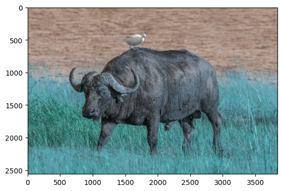
img1 = cv2.imread('./Img/African_buffalo.jpg')

print("Shape of image is ",img1.shape)
print("Max value of image is ",img1.max())
print("Min value of image is ",img1.min())

Shape of image is  (2560, 3840, 3)
Max value of image is  255
Min value of image is  0

cv2.imshow function can be used to load an image from CLI, with native GUI.
In Jupyter Notebook env, cv2.imshow will not work so we can preview the image using matplotlib.imshow

import matplotlib.pyplot as plt
plt.imshow(img1)
plt.axis('off')
plt.show()

OCV

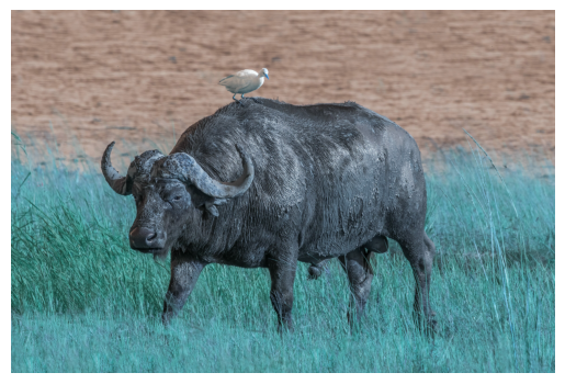
Save img to another image using cv2.imwrite

cv2.imwrite("./Img/African_buffalo_copy.jpg", img1)

Upscale and Downscale image

The function cv2.resize() is used to resize an image. It takes the following parameters:
- src: The source image.
- dsize: The desired size of the output image. It is a tuple (width, height).
- fx: The scale factor along the horizontal axis. If it is 0, it is calculated as (dsize.width / src.width).
- fy: The scale factor along the vertical axis. If it is 0, it is calculated as (dsize.height / src.height).
- interpolation: The interpolation method to be used. It can be one of the following:
  - cv2.INTER_NEAREST: Nearest neighbor interpolation.
  - cv2.INTER_LINEAR: Bilinear interpolation (default).
  - cv2.INTER_AREA: Resampling using pixel area relation. It may be a preferred method for image decimation, as it gives moire’-free results. But when the image is zoomed, it is similar to the INTER_NEAREST method.
  - cv2.INTER_CUBIC: Bicubic interpolation over 4x4 pixel neighborhood.
  - cv2.INTER_LANCZOS4: Lanczos interpolation over 8x8 pixel neighborhood.

img1_downsize = cv2.resize(img1, (img1.shape[1]//2, img1.shape[0]//2),interpolation=cv2.INTER_LINEAR)
print("Shape of downsize image is ",img1_downsize.shape)

Shape of downsize image is  (1280, 1920, 3)

img1_upsize = cv2.resize(img1, (img1.shape[1]*2, img1.shape[0]*2),interpolation=cv2.INTER_CUBIC)
print("Shape of upsize image is ",img1_upsize.shape)

Shape of upsize image is  (5120, 7680, 3) ### Cropping image - Using sliding window to crop the image

img1_cropped = img1[100:400, 100:400]
print("Shape of cropped image is ",img1_cropped.shape)
plt.imshow(img1_cropped)

Shape of cropped image is  (300, 300, 3) 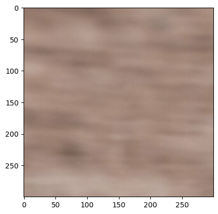![crop](/assets/img/project/OpenCV_tutorial1_13_2.png)

Image translation and rotation

Some popular function:

cv2.ROTATE_90_CLOCKWISE
cv2.getRotationMatrix2D
cv2.warpAffine

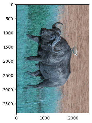
img1_rotated = cv2.rotate(img1, cv2.ROTATE_90_CLOCKWISE)
plt.imshow(img1_rotated)

png

Convolution

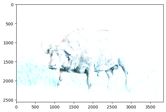
In Computer Science, convolution is a mathematical operation that combines two functions to produce a third function. In the context of image processing, convolution is used to apply filters to images, which can enhance certain features or reduce noise. The process involves sliding a kernel (a small matrix) over the image and performing element-wise multiplication and summation to produce a new pixel value in the output image. This technique is fundamental in various applications such as edge detection, blurring, and sharpening of images.
In OpenCV, we can apply function cv2.filter2D to apply convolution to an image
The example below is to apply a blur kernel to existing image

import numpy as np
kernel_blur = np.ones((5,5),np.float32)/5
img_blur = cv2.filter2D(img1, ddepth=-1, kernel=kernel_blur)
plt.imshow(img_blur)

png

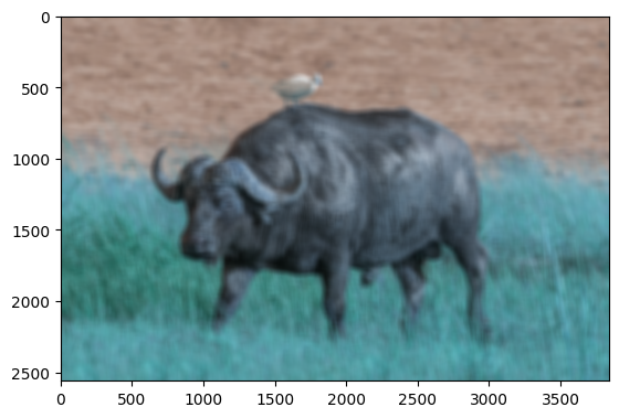
We can also use cv2.blur instead of cv2.filter2D

img_blur2 = cv2.blur(img1, ksize=(50,50))
plt.imshow(img_blur2)

png

Alternatively, we can apply sharp kernel to original image:

kernel_sharp = np.array([[0, -1,  0],
                         [-1,  5, -1],
                         [0, -1,  0]])
img_sharp = cv2.filter2D(img1, ddepth=-1, kernel=kernel_sharp)
plt.imshow(img_sharp)

jpg